Introduction to Reinforcement Learning for Absolute Beginners
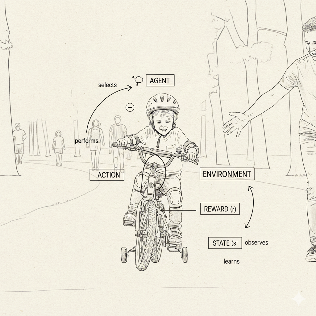 Image: A child learning to ride a bicycle through trial and error - the essence of reinforcement learning
Imagine teaching a child to ride a bicycle. They learn by trying, wobbling, and maybe falling – trial and error guided by little victories and tumbles. Over time, they adjust their balance and steering to maximize the thrill of coasting (and minimize the painful falls). This process of trial-and-error learning is exactly what reinforcement learning (RL) is all about. In RL, a computer agent learns from feedback: it takes actions, observes the outcomes (rewards or penalties), and adapts its behavior to get better results in the future. Just as you might avoid actions that make a puppy grumpy and repeat those that make it wag its tail, an RL agent learns to favor actions that lead to positive rewards.
Reinforcement learning stands out in the AI world because it mimics how humans and animals actively learn from experience. It doesn’t rely on being told the “right answer” for each situation (as in supervised learning); instead, it explores different actions and infers which strategies work best through feedback. The goal of an RL agent is to maximize cumulative reward over time – somewhat like game players trying to rack up the highest score or athletes tweaking their moves to win races. In practice, RL has enabled impressive feats: a computer learned to play the ancient game of Go at superhuman levels (AlphaGo), robots are learning to walk over rough terrain, and recommendation systems are tuning themselves to improve engagement. In this article, we’ll unpack RL’s core ideas – agent, environment, rewards, policies, value functions, and more – using friendly analogies (think game players, pet robots, and even dancing cars). By the end, you’ll have a solid conceptual grasp of RL and be inspired to take your own RL “first ride” in code or simulation.
The Agent-Environment Loop: How RL Works
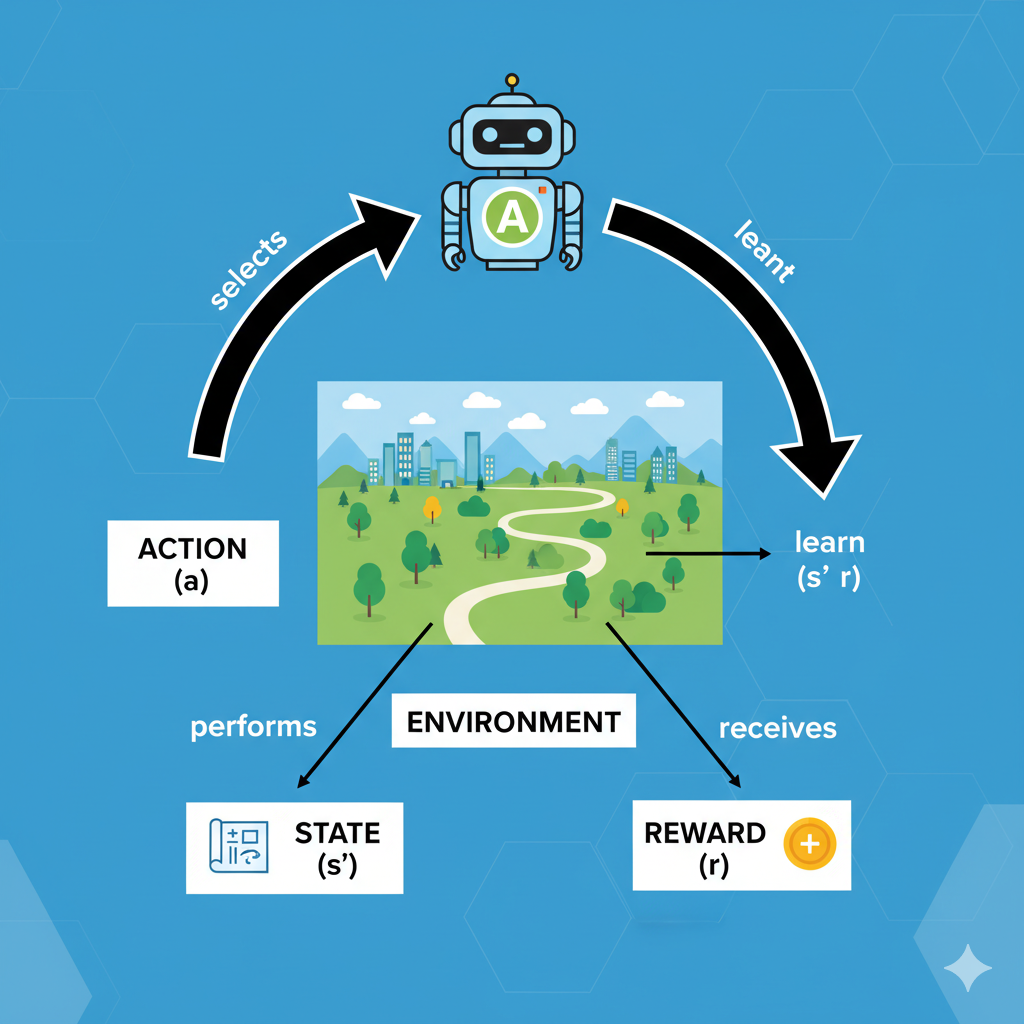 Image: The fundamental RL loop showing agent-environment interaction
At the heart of reinforcement learning is an agent interacting with an environment. The agent can be anything making decisions (a robot, software program, game player, etc.), and the environment is everything it interacts with (the world, game, simulation, etc.).
Every moment, the agent observes the current state of the environment, chooses an action, and then the environment responds by moving to a new state and giving the agent a reward (a numeric score or signal). This cycle repeats over and over.
🔄 The RL Process in 4 Simple Steps:
Step 1: At time
t, the agent observes the current StateS_tStep 2: The agent selects an Action
A_tto performStep 3: The environment transitions to a new State
S_{t+1}and provides a RewardR_{t+1}Step 4: The agent observes
(S_{t+1}, R_{t+1})and decides on the next action
📝 This creates a continuous learning loop where the agent improves its decisions over time!
This is often drawn as the agent-environment loop: the agent acts on the environment, and the environment “feeds back” a new state and reward. The agent’s goal is to choose actions (over many steps) that maximize the total sum of rewards it gets. In other words, it’s trying to figure out which behavior yields the biggest payoff in the long run. This is akin to a video-game player learning that certain moves earn more points over time, or a pet learning that certain tricks earn treats.
One helpful analogy is to think of yourself and your pet dog: you (the agent) can pet, feed, or play with your dog (the actions). The dog (the environment) responds: wagging its tail or licking you (a positive reward), or maybe barking or nipping (a negative signal). You adjust your behavior to maximize the good responses. Over time you learn, for example, “whenever I do this (like throw a ball), I get a happy tail wag!” Similarly, the agent learns, “if I do this action in that situation, I tend to get a higher reward”. The core loop of RL – action, state change, reward – lets the agent discover which sequences of actions work best.
Importantly, RL doesn’t tell the agent explicitly which action is correct. Instead, the agent figures it out through experience. As one introduction notes, “RL teaches an agent to interact with an environment and learn from the consequences of its actions”. In supervised learning you have example answers; in RL the agent experiments and sometimes makes “mistakes”, learning indirectly by seeing which choices lead to higher rewards. This makes RL especially powerful for problems where you can try things out but can’t easily write down the correct answer in advance – for example, balancing an inverted pendulum, trading stocks, or teaching an AI to play a strategy game.
📚 Essential RL Vocabulary
These key terms will appear throughout our journey - think of them as your RL dictionary!
| Term | Symbol | Definition |
|---|---|---|
| 🤖 Agent | - | The learner or decision maker (software or robot) |
| 🌍 Environment | - | What the agent interacts with (game, maze, real world, etc.) |
| 📍 State | S | A description of the current situation (robot’s position, game board, etc.) |
| 🎯 Action | A | A choice the agent can make (move left/right, speak a phrase, etc.) |
| 🏆 Reward | R | A numerical score after taking an action (positive = good, negative = bad) |
| 🧠 Policy | π | The agent’s strategy for mapping states to actions |
| 💎 Value | V | A measure of how “good” a state is for future rewards |
💡 Think of it like this: The Agent (you) interacts with the Environment (a video game), observes the State (current level), takes Actions (move, jump, shoot), receives Rewards (points, lives), and develops a Policy (strategy) to maximize Value (high score)!
These fit into a framework called a Markov Decision Process (MDP), which formalizes RL mathematically. An MDP is defined by a set of states (S), actions (A), transition probabilities, reward rules, and a discount factor γ (see below). But you can understand RL quite well with just the intuitive idea of states, actions, and rewards forming a loop.
States, Actions, and Rewards
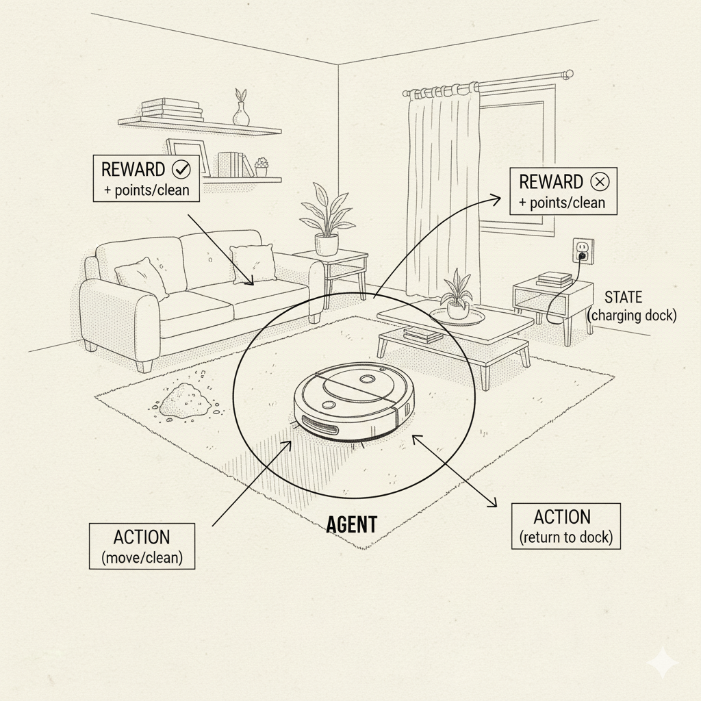 Image: A robot vacuum demonstrating states, actions, and rewards in a real environment
🧩 Breaking Down the Core Components
📍 State (S) - “Where am I and what’s happening?”
The state is like a snapshot of the current situation that tells the agent everything it needs to know to make a decision.
Examples:
- 🤖 Robot vacuum: Current location + dirt sensor readings + battery level
- ♟️ Chess game: Positions of all pieces on the board
- 🚗 Self-driving car: Speed, location, traffic conditions, weather
💡 Key insight: States should have the Markov Property - the future depends only on the current state, not how we got there!
🎯 Action (A) - “What can I do next?”
Actions are the moves available to the agent in any given state.
Examples:
- 🤖 Robot vacuum: {Move Forward, Turn Left, Turn Right, Start Cleaning}
- ♟️ Chess: {Move Pawn, Move Knight, Castle, etc.}
- 🚗 Self-driving car: {Accelerate, Brake, Turn Left, Turn Right, Change Lane}
🧠 The agent’s Policy
πis like its “brain” - it decides which action to pick in each state!
🏆 Reward (R) - “How well did I do?”
Rewards are the feedback scores that tell the agent if its actions were good or bad.
Examples:
- ✅ Positive: +10 for reaching goal, +1 for cleaning dirt, +5 for winning a game
- ❌ Negative: -10 for crashing, -1 for wasting time, -5 for losing
- 🔄 Neutral: 0 for neutral actions
🎯 Goal: Maximize the total reward over time (not just immediate reward!)
The agent doesn’t just care about the immediate reward; it cares about future ones too. For example, you might take a slightly negative step now because it leads to a big positive reward later (like sacrificing a pawn in chess to win the game). To handle this, RL uses the idea of discounting. A discount factor γ (gamma) between 0 and 1 determines how much the agent values future rewards compared to immediate ones. A simple view: if γ=0.9, a reward received one step later counts as 90% as important as a reward now, two steps later as 81%, and so on. This captures the intuition that immediate rewards are often more certain or valuable, but it still takes future outcomes into account.
🔢 The Mathematical Foundation (MDP)
Don’t worry - these equations just formalize what we already understand intuitively!
📋 Formal Definition of MDP:
| Symbol | Meaning | Think of it as… |
|---|---|---|
S | Set of all possible states | All possible “situations” in our world |
A | Set of all possible actions | All possible “moves” the agent can make |
| **`P(s' | s,a)`** | Transition probability |
R(s,a) | Immediate reward function | “How many points do I get for this action?” |
γ | Discount factor (0≤γ≤1) | “How much do I care about future vs. now?” |
🎯 The Ultimate Goal:
Maximize: E[Σ(γ^t × R_t)] from t=0 to ∞
Translation: Find the strategy that gets the highest total score over time!
💡 Discount Factor Intuition:
γ = 0: “I only care about immediate rewards” (very short-sighted)γ = 0.9: “Future reward worth 90% of current reward” (balanced)γ = 1.0: “All future rewards equally important” (very long-term thinking)
💡 Fun Fact: The word “reinforcement” comes from psychology, where rewarding an animal or person for a behavior is called reinforcement. Pavlov’s famous dogs (learning to salivate to a bell after hearing it repeatedly with food) is conceptually similar to RL: behaviors are reinforced (encouraged) by rewards and discouraged by punishments. In RL, rewards play the role of reinforcing signals, guiding the agent toward better behavior.
Policies and Value Functions
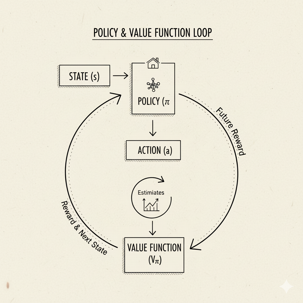 Image: Visualization of how policies map states to actions and value functions estimate future rewards
🧠 The Two Pillars of RL Intelligence
🎮 Policy (π) - “The Agent’s Strategy Playbook”
A policy is like the agent’s decision-making rulebook that tells it what to do in every situation.
🎯 Types of Policies:
📖 Deterministic Policy: “In state
S, always do actionA”- Example: “When facing a wall, always turn right”
🎲 Stochastic Policy: “In state
S, do actionAwith 70% probability, actionBwith 30%”- Example: “When enemy approaches, attack 80% of time, defend 20% of time”
💎 Value Functions - “The Agent’s Crystal Ball”
Value functions are the agent’s way of predicting the future - “How good is this situation?”
| Function | Symbol | What it answers |
|---|---|---|
| State Value | V^π(s) | “How good is this state overall?” |
| Action Value (Q-Function) | Q^π(s,a) | “How good is taking this specific action?” |
🔮 Real Example:
V^π(near goal) = 50→ “Being near the goal is worth 50 points!”Q^π(near wall, move forward) = -10→ “Moving forward near a wall loses 10 points!”
For example, if V^π(s)=10, it means under policy π the agent expects to collect 10 reward points in total (discounted) from state s onward. If Q^π(s,a)=8, taking action a in s and then following the policy is worth 8 points. Once the agent knows these values, it can behave better. In fact, if it finds the optimal values (V* or Q*), it can choose the action that maximizes expected future reward: “take the action with the highest Q*(s,a)”. Reinforcement learning algorithms often focus on estimating these value functions through experience.
Why do we care about values? Because they provide a way for the agent to compare actions. Imagine the agent is in a state and has two choices: move left or right. If it had a table of Q-values, it could see “if I go left I expect +5 reward eventually, if I go right I expect +3”. Then it’ll go left. Learning good value estimates is at the heart of many RL methods.
⚡ The Bellman Equation: The Heart of RL
The Bellman Equation is like RL’s most important recipe - it connects current and future rewards!
🧮 The Magic Formula:
V^π(s) = E[R(s,a) + γ × V^π(s') | s]
🗣️ In Plain English:
“The value of where I am now = What I get immediately + (Discounted) value of where I’ll be next”
🎯 Breaking it down:
- Current reward:
R(s,a)→ Points I get right now - Future value:
γ × V^π(s')→ Expected future points (discounted) - Total value: Current + Future → Complete picture!
💡 Why This Matters: This recursive relationship is how agents learn to look ahead and make smart long-term decisions instead of just chasing immediate rewards!
Importantly, in optimal RL, we want the optimal value functions V* or Q*. These satisfy the Bellman optimality equations, where we pick the maximum over next actions. But you don’t need to dive into those details yet. What matters is that value functions let the agent reason about long-term payoff rather than just immediate reward.
Exploration vs. Exploitation
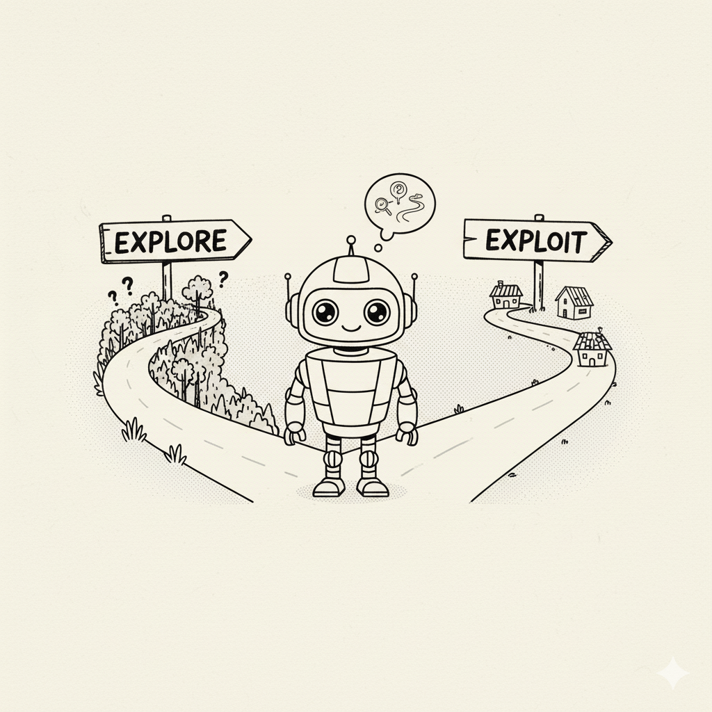 Image: A robot at crossroads choosing between exploring new paths or exploiting known good paths
🤔 The Great RL Dilemma: Explore or Exploit?
One of RL’s biggest challenges is deciding: “Should I stick with what I know works, or try something new?”
| 🔍 EXPLORE | 💰 EXPLOIT |
|---|---|
| Try new, unknown actions | Use known good actions |
| Might discover something amazing | Guaranteed decent results |
| Risk: Could waste time on bad choices | Risk: Miss out on better options |
| “Let me try that new restaurant!” | “I’ll stick with my favorite restaurant” |
🍦 The Ice Cream Stand Analogy
Imagine you’re at an ice cream stand with 3 flavors:
- ✅ Vanilla: You’ve tried it, pretty good (7/10)
- ✅ Chocolate: You’ve tried it, okay (6/10)
- ❓ Strawberry: Never tried - could be amazing (10/10) or awful (2/10)
What do you choose? This is the exploration-exploitation dilemma!
🎯 The ε-Greedy Solution
A popular strategy that balances both:
- 90% of the time (
1-ε): Pick the best known action (exploit) - 10% of the time (
ε): Try a random action (explore)
📈 Smart Strategy: Start with high exploration (
ε = 0.3) when learning, then gradually reduce it (ε = 0.1) as you gain experience! Wikipedia explains: “the focus is on finding a balance between exploration (of uncharted territory) and exploitation (of current knowledge) with the goal of maximizing the cumulative reward”.
🧩 Try This: Imagine a simple grid world where an agent can move up/down/left/right for rewards. How would you balance exploration vs. exploitation? One idea: start with high exploration (ε large) and gradually reduce it as your agent becomes more confident. Try coding a tiny example in Python or on pen-and-paper to see how a greedy strategy versus an exploratory strategy might perform.
Learning Algorithms (Conceptual Overview)
With these basics in place, let’s outline how an agent actually learns. Many RL algorithms exist, but we’ll focus on a few intuitive classes.
Value-Based Methods: Q-Learning and SARSA
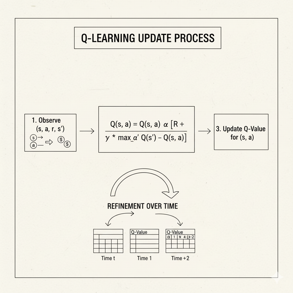 Image: Visual representation of Q-Learning update process showing how Q-values are refined over time
Value-based methods center on learning value functions (usually the action-value Q(s,a)) and deriving a policy from them.
Q-Learning is one of the most famous algorithms. It learns a table (or function) of Q(s,a) values by repeatedly updating them based on experience. At each step, if the agent is in state s, takes action a, receives reward r, and lands in state s', Q-learning updates:
Q(s,a) ← Q(s,a) + α(r + γ × max Q(s',a') - Q(s,a))
                              a'
where α is a learning rate. Intuitively, Q-learning says, “take the current Q(s,a) and move it partway toward the sum of the immediate reward r plus the best possible future reward max Q(s',a') (discounted)”. Notice it uses the maximum over next actions a', meaning it assumes the agent will behave optimally from state s' onward. This makes Q-learning off-policy: it learns about the best possible strategy regardless of what actions it actually took during learning. In practice, the agent might explore randomly, but Q-learning still updates the Q values as if the agent had taken the best action. Over many trials, Q(s,a) values converge to the optimal values, letting the agent choose the action with the highest Q in each state (that is the optimal policy).
SARSA (State-Action-Reward-State-Action) is similar but on-policy. Its name reflects how it updates: it considers the sequence (s, a, r, s', a'). After observing (s,a,r,s') and then the agent picks next action a' according to its current policy, SARSA updates:
Q(s,a) ← Q(s,a) + α(r + γ × Q(s',a') - Q(s,a))
The key difference is that SARSA uses Q(s', a') – the value of the actual next action a' the agent took (following its behavior) – whereas Q-learning uses max Q(s', a') (the best possible action). As GeeksforGeeks notes, “Q-learning is an off-policy method meaning it learns the best strategy without depending on the agent’s actual actions… SARSA is on-policy, updating its values based on the actions the agent actually takes”. In plain terms, Q-learning chases the optimal policy regardless of exploration, while SARSA updates according to whatever policy (including randomness) the agent is following. SARSA tends to be “safer” if random exploratory moves are dangerous, because it keeps track of the actual behavior.
Both Q-learning and SARSA rely on the Bellman update concept to iteratively improve estimates of Q(s,a). They need a table of values if states and actions are small and discrete. For large or continuous spaces, function approximation (like neural networks) or lookup tricks are needed.
Policy-Based Methods: Policy Gradients
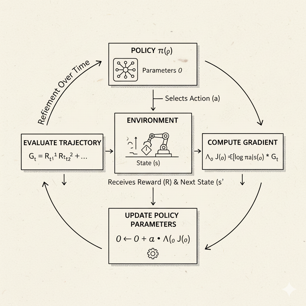 Image: Visualization of policy gradient learning process showing how policy parameters are updated
Instead of focusing on values, policy-gradient methods directly search for a good policy. Here the agent’s policy is typically represented by a parameterized function (for example, a neural network with weights θ that outputs action probabilities). The objective is to maximize the expected reward by adjusting those parameters in the direction that increases the chance of high-reward actions.
In essence, policy-gradient algorithms try to compute the gradient of expected reward with respect to the policy parameters and then perform gradient ascent. A classic simple example is the REINFORCE algorithm, where the update nudges the policy to make actions that led to high returns more likely. One benefit is that policy methods naturally handle continuous or large action spaces and stochastic policies. According to Wikipedia: “Policy gradient methods… directly maximize the expected return by differentiating a parameterized policy”. Unlike value-based methods (which learn a V or Q function and derive a policy), policy-gradient (aka policy optimization) learns the policy directly “without consulting a value function”. (Often, more advanced methods like actor-critic combine both: the “actor” is a policy gradient, and the “critic” learns a value function to reduce variance.)
Example: Suppose your policy network outputs a probability distribution over actions. If a chosen action later results in high reward, you slightly increase the probability of that action in the future. If it yields low reward, you decrease its probability. Over many episodes, the policy gets “tuned” toward actions yielding higher returns.
Other Algorithm Types
There are many more RL approaches (e.g. Temporal-Difference (TD) learning, Monte Carlo methods, actor-critic algorithms). TD learning (like SARSA/Q-learning) updates estimates using one-step lookahead and the Bellman idea, whereas Monte Carlo averages complete episodes. Actor-critic methods combine policy and value approaches: the actor (policy) suggests actions and the critic evaluates them. We won’t go into all these, but keep in mind the landscape is rich. For an absolute beginner, focusing on the intuitive ideas behind Q-Learning, SARSA, and policy-gradient is plenty to start with.
Bellman Equations and Discounting (Math Intuition)
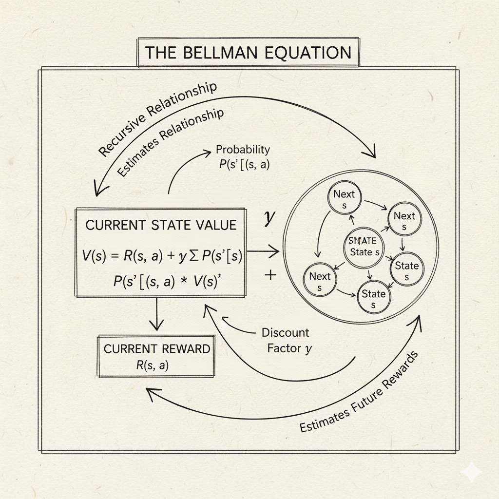 Image: Visual representation of the Bellman equation showing the recursive relationship between current and future values
To understand why these algorithms work, it helps to see the Bellman equations again, at least intuitively. The idea is that the value of a state (or state-action) depends on rewards and the values of successor states. For example, the Bellman optimality equation for the state-value function V*(s) is:
V*(s) = max [R(s,a) + γ × Σ P(s'|s,a) × V*(s')]
        a           s'
In words: “the best possible expected reward from state s equals the best action a you can take now, receiving immediate reward R(s,a) plus the discounted value of the next state.” A similar form holds for Q*(s,a). We won’t solve these by hand, but they justify why, for instance, Q-learning uses the max Q(s',a') term in its update rule – it’s implementing this Bellman optimality idea incrementally. The GeeksforGeeks RL guide puts it simply: “the Bellman Equation says the value of a state is equal to the reward received now plus the expected value of the next state”.
The discount factor γ figures in here to weigh immediate versus future reward. A γ close to 0 means the agent is short-sighted (mostly cares about immediate reward), while γ near 1 means it values future rewards almost as much as immediate ones. You can picture a timeline of rewards: receiving 10 points now and 0 later versus receiving 0 now and 10 later. With discounting, 10 later is worth less (10×γ) in today’s terms. Setting γ balances whether the agent should focus on quick gains or on long-term strategy. Many problems use γ around 0.9 or 0.99 to give significance to future rewards while ensuring the math converges.
Exploration Example: Multi-Armed Bandits
 Image: A row of slot machines representing the multi-armed bandit problem
A useful sub-problem in RL is the multi-armed bandit scenario. Imagine a row of slot machines (one-armed bandits) each with unknown payout probabilities. You have to figure out which machine to play to maximize total winnings. You might first explore each machine to estimate its payout and then exploit the best one. This captures the core exploration-exploitation tradeoff.
The analogy to reinforcement learning is straightforward: each slot machine is an action, and pulling it yields a stochastic reward. The goal is to identify the “best arm” quickly. As a real-world analogy, consider you’re trying to find your dog’s favorite treat. You have 7 new brands. You give your dog a different one each day and see how it reacts. Maybe Brand A got a huge tail wag on one day, but the dog might have been excited for another reason. To be sure, you need to try each brand multiple times to estimate its average appeal. Then you want to focus on the top few favorites and avoid the worst ones (regret minimization).
This is exactly what bandit algorithms do. A naive approach (“try each brand n times and pick the best average”) works but is wasteful. Smarter algorithms (like Upper Confidence Bound, Thompson Sampling, ε-greedy) try to reduce unnecessary “unpleasant experiments” by balancing exploration with focusing on promising arms. In RL jargon, bandits are the single-step (no state changes) version of RL, highlighting the exploration problem. Understanding bandits can help you build intuition before tackling full multi-step RL.
💡 Fun Fact: The “multi-armed bandit” name comes from imagining a gambler in a casino with many slot machines (“one-armed bandits”). You want to figure out which arm to pull to win the most, balancing trying new machines (exploration) and sticking with high-reward machines (exploitation).
Real-World Case Study: AlphaGo (Game Playing)
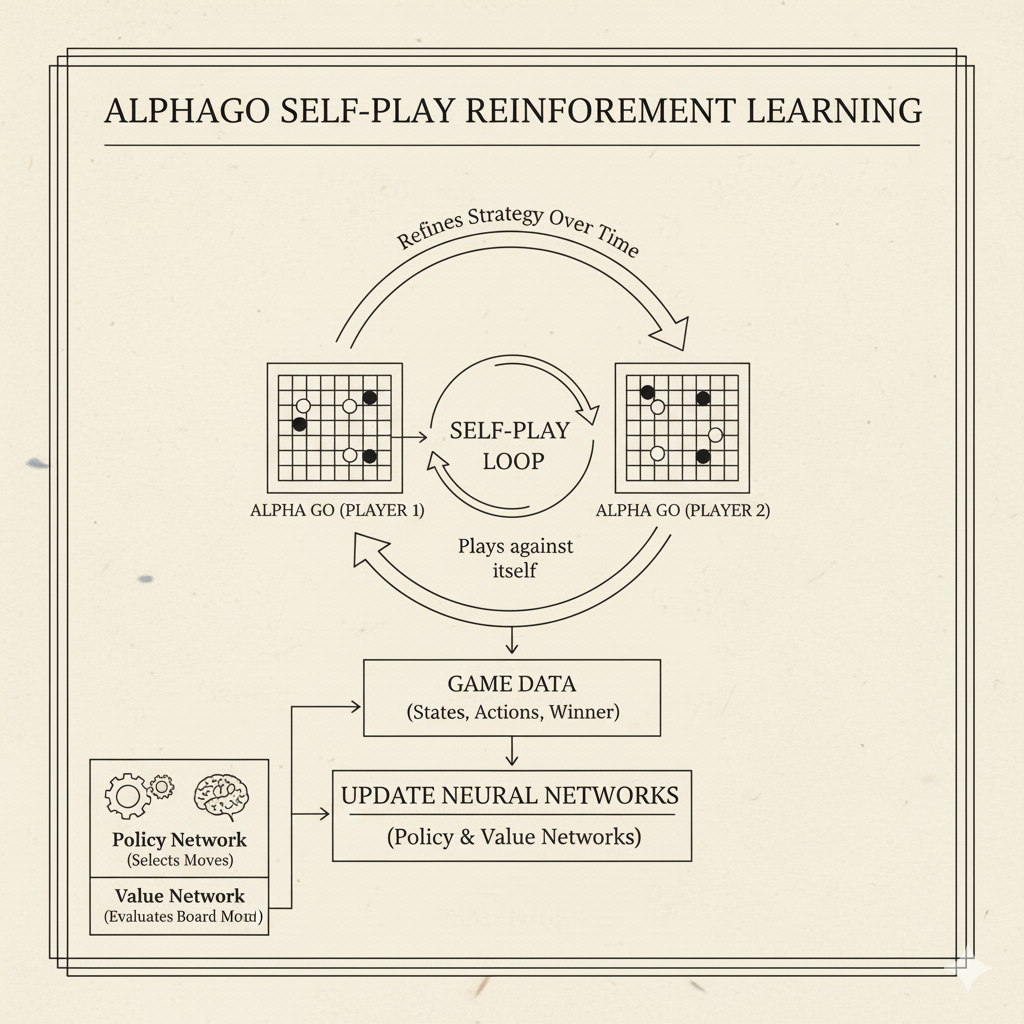 Image: AlphaGo training process showing self-play reinforcement learning
One of the most famous successes of reinforcement learning is AlphaGo, developed by DeepMind. Go is an ancient board game of staggering complexity (even more complex than chess). In 2016, AlphaGo became the first computer program to defeat a human world champion at Go, stunning the world. How did it learn to do this?
AlphaGo combined deep neural networks with reinforcement learning and search. It had a policy network (to select moves) and a value network (to evaluate board positions). First, it learned from human games (“supervised learning” pre-training), giving it a good initial sense of reasonable moves. Then the key step was self-play reinforcement learning. AlphaGo played millions of games against copies of itself. Each game provided a sequence of states, actions, and a final winner (reward). Through these games, it improved its neural networks via RL: effectively it tried actions (moves), observed win/loss outcomes, and adjusted its strategy to maximize its chance of winning (reward). As DeepMind reports, “we instructed AlphaGo to play against different versions of itself thousands of times, each time learning from its mistakes — a method known as reinforcement learning. Over time, AlphaGo improved and became a better player.”
This is a powerful illustration of RL’s trial-and-error at scale: AlphaGo didn’t have a human telling it exactly which move is best; it discovered strong moves by playing repeatedly. The result was creative strategies unseen before. Lee Sedol, a top Go champion, famously said of a move AlphaGo played, “I thought AlphaGo was based on probability calculation… But when I saw this move, I changed my mind. Surely, AlphaGo is creative.” The key takeaway: RL enabled an AI to explore a vast game space and learn strategic patterns just by chasing the long-term reward of winning.
⚙️ Real Example: Many video games and board games can be posed as RL problems. You could try writing a simple RL agent for Tic-Tac-Toe or Connect Four. In Python, using libraries like OpenAI Gym (for classic games/environments) and stable-baselines, beginners often train an agent to solve CartPole balancing or play Pong using Q-learning or a policy gradient. Seeing an agent gradually improve at a small game is hugely motivating.
Real-World Case Study: Robotics and Locomotion
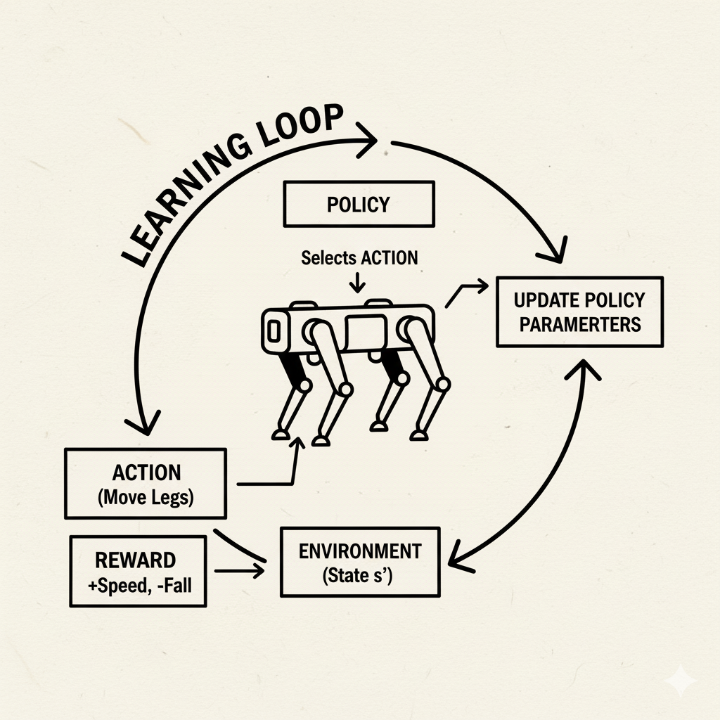 Image: Boston Dynamics robot learning locomotion through reinforcement learning
Reinforcement learning has proven especially powerful in robotics, where traditional programming of behaviors is hard. Instead of manually coding every movement, engineers let RL discover controllers. A great example is Boston Dynamics’ work with their Spot robot dog.
Historically, Spot’s walking gait was generated by carefully engineered control algorithms. Boston Dynamics showed that RL offers an alternative: learn the walking policy in simulation. As their blog explains, RL is “an alternative approach to programming robots that optimizes the strategy (controller) through trial and error experience in a simulator”. In practice, they define a reward function (e.g. “walk without falling”), simulate many varied terrain scenarios, and let a neural-network policy learn to control the robot’s joints. Millions of simulated trials yield a policy that can handle stairs, slippery floors, or rough ground. This learned policy is then tested on real robots and refined. The result? Spot can now walk faster and more robustly over uneven ground than the old hand-coded version.
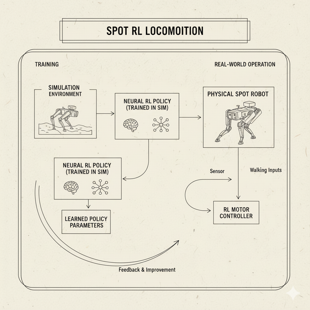 Block diagram from Boston Dynamics: a neural “RL policy” is trained in simulation and then combined with Spot’s existing path planner. The policy takes sensor inputs and outputs walking commands optimized via reinforcement learning
This robotic example illustrates two strengths of RL: (1) it can handle complex, dynamic tasks (walking is tricky!), and (2) it can exploit simulation. Gathering millions of trials on a real robot would be impractical (and dangerous); instead, engineers simulate diverse environments. RL algorithms thrive on simulated data, learning strategies that transfer to the real world. Beyond Spot, many researchers have used RL to teach robots to pick up objects, balance on one leg, or even fly.
Real-World Case Study: Recommender Systems
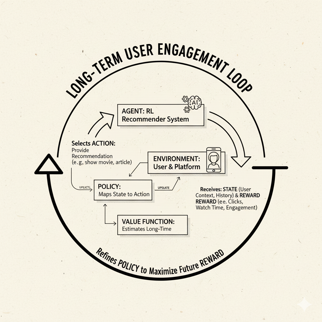 Image: Recommender system using RL to optimize long-term user engagement
Recommender systems (like those on YouTube, Netflix, Amazon) suggest items to users (videos, products, etc.). Traditionally, these use supervised learning or heuristics (“users who liked X also liked Y”). But RL offers a way to optimize for long-term engagement rather than one-off clicks. For instance, Google reported using RL to improve YouTube recommendations.
In that YouTube example, engineers replaced the existing search-based recommendation with an RL agent. The agent observed user clicks (rewards) and adjusted its recommendation policy over time. The RL approach “quickly matched the performance of the current implementation. After a little more time it surpassed it”. This is notable because Google’s recommendation algorithms are already world-class; yet an RL system, with relatively little hand-tuning, learned an even better strategy purely from user feedback.
In simpler terms, think of a recommender as an agent choosing which video to show a user. Each recommendation (action) yields feedback: perhaps the user watches the video (reward) or not (no reward or even a small penalty). The agent’s goal is to maximize total watch time over a session or long-term. RL models are well-suited because they can explicitly account for sequential effects (if you recommend a low-quality video now, the user might leave early, hurting future rewards). Recent research uses RL to personalize recommendations by treating them as actions in an MDP. While building these systems is complex, the core idea is: optimize recommendations by trial, feedback, and gradual improvement.
⚙️ Real Example: As a beginner project, you might try an RL formulation of the “Multi-Armed Bandit” for news article recommendation. Imagine a set of 5 headlines; choosing one randomly yields a click or not. Let an RL agent learn which headlines to show to maximize clicks, balancing new headlines and popular ones.
The Learning Process: Putting It All Together
Let’s summarize what an RL learning loop might look like in practice:
Initialize: Define the state space, action space, and reward function. Choose a learning algorithm (e.g. Q-learning, policy gradient).
Observe State: The agent starts in some state $S_0$.
Select Action: According to its current policy (which might start random or partial), it chooses action $A_0$ (often using some exploration strategy like ε-greedy).
Apply Action: The action is executed in the environment (or simulation).
Receive Feedback: The environment returns a reward $R_1$ and new state $S_1$.
Update Knowledge: The agent updates its policy or value estimates using this experience. For example, it might update $Q(S_0,A_0)$ using the Bellman rule, or adjust policy parameters via gradient descent.
Repeat: The agent moves to $S_1$, picks $A_1$, and so on. Over many steps (and episodes, which are sequences of steps ending in a terminal state), it continually refines its policy.
This process continues until the policy performs well (maximizing reward) or training time runs out. The “learning” happens gradually: first the agent is naive, often performing poorly; but with enough trials it accumulates knowledge (values or policy gradients) and becomes competent.
In simpler problems (small discrete states), you might even visualize a Q-table. For a grid world, imagine a table with rows as states and columns as actions, each cell showing $Q(s,a)$. As learning proceeds, you would see this table’s values change (often pictured as a heatmap of values) until higher (hot) values align with the best actions. In more complex tasks, deep neural nets approximate these values or policies.
Putting Concepts into Practice
As an aspiring RL practitioner, here are some tips and resources:
Get your hands dirty: Use platforms like OpenAI Gym (a library of RL environments) to experiment. OpenAI Gym provides classic control tasks (CartPole, MountainCar) and games. You can code up simple Q-learning or use libraries like Stable Baselines to try advanced algorithms.
Google Colab notebooks: Many tutorials share Colab links. For example, look up “CartPole Q-learning Colab” or “DQN Atari Colab”. Running code and seeing results will cement understanding.
RL Book (Sutton & Barto): “Reinforcement Learning: An Introduction” by Sutton and Barto is the bible of RL. It’s free online and packed with insight (though it can be mathy).
RL Communities: Join forums or groups (e.g. r/reinforcementlearning on Reddit, GitHub RL projects, or LinkedIn communities). Learning from others’ questions and code is invaluable.
Try simple projects: Aside from game environments, try guiding a robot vacuum in simulation, or balancing a pole, or even something like tic-tac-toe. Each new domain reinforces the key ideas in a fun context.
Fun challenge: Build a small bandit solver (like our multi-flavor dog analogy) and compare strategies (ε-greedy, UCB, softmax). See how quick each learns the best arm.
🧩 Try This: A classic beginner project is the CartPole balancing task. The agent must balance a pole on a cart by moving left or right. It’s fully observable and simple. Implement a Q-learning agent with a table (discretize the state) or a policy gradient. Watch how after many trials it learns to balance longer and longer.
Conclusion and Next Steps
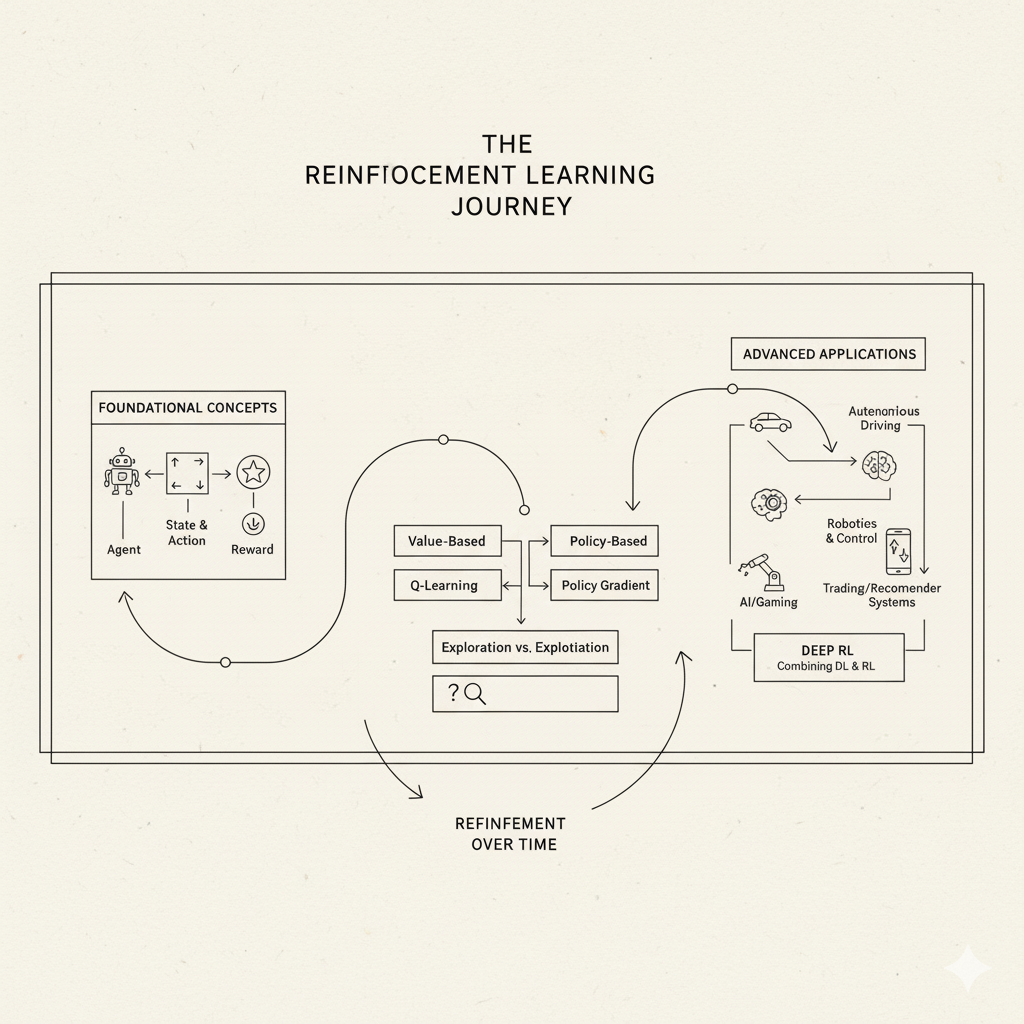 Image: Visual summary of the reinforcement learning journey from basics to advanced applications
Congratulations – you’ve taken your first steps into the exciting world of reinforcement learning! We started with the simple idea of learning by trial and error (just like a child learning to ride a bike), introduced the core components (agent, environment, states, actions, rewards, policies), and built up to how algorithms like Q-learning and policy gradients really work. We saw analogies (dogs, slot machines, games) and real-world examples (AlphaGo, robot dogs, YouTube recommendations) that show how RL enables learning complex behaviors through experimentation.
If there’s one big takeaway, it’s this: Reinforcement learning is about learning by doing. You define a problem as a series of decisions, give your agent rewards for good outcomes, and let it try, fail, and improve. Over time, even very hard tasks become doable because the agent learns from experience.
Next Steps: To keep momentum, pick a small project or tutorial to try. Perhaps train an RL agent on a classic Gym environment (CartPole, MountainCar, or a simple maze). Read a chapter of Sutton & Barto on something that interests you (e.g. policy gradients, actor-critic, or multi-agent RL). Explore courses or YouTube lectures on RL. Join an online community and ask questions – fellow learners can share advice and code.
Above all, stay curious and patient. RL can be challenging, but it’s also incredibly powerful. Every great AI breakthrough in games, robotics, or beyond started with this simple loop of action, reward, learn. Now it’s your turn to dive in and let trial-and-error learning guide you to new discoveries. Happy learning, and enjoy your first RL adventures!
💡 Final Tip: Reinforcement learning often involves tuning and tweaking. Don’t be discouraged if initial attempts fail. Each “failure” is informative feedback. With perseverance and clever rewards, your agent will find its way. As AlphaGo’s story shows, what looks impossible can become possible through trial, error, and learning. Good luck, and have fun exploring the world of RL!
Sources: Authoritative RL resources and case studies were used for this introduction. These detail core RL definitions, equations, and real examples. Each concept above is grounded in the literature and high-quality tutorials for newcomers.